图像分类任务
目标:有一个固定分类标签的集合,输入一张图像,从标签集合中找到与图像对应的标签分配给输入图像。
问题: 计算机看到的图像与人眼不同,彩色图像在计算机中只是存储RGB三信道像素值的数据结构。

- 挑战:
- Viewpoint variation 视角变化
- Illumination 光照变化
- Deformation 形变
- Occlusion 遮挡
- Background Clutter 背景干扰
- Intraclass variation 类别间差异:同一类物体之间存在差异
- 数据驱动方式(Data-Driven Approach):
- 收集图像和标签的训练集
- 使用机器学习方法训练分类器
- 用分类器预测新图像的标签,并作出评价。
Nearest Neighbor分类器
算法思想
k-Nearest Neighbor算法感觉是一种非常暴力的算法,对于给定的测试集,遍历所有训练集,找到与训练集最接近的k个样本,最近的k个样本进行“投票”——即找到最近k个样本中出现次数最多的标签,并分配给该测试数据。
距离度量的选择
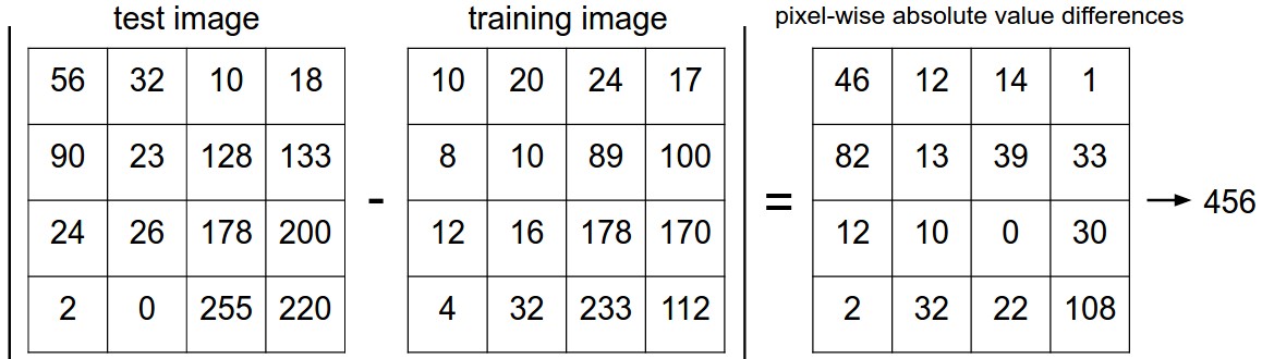
上述思想涉及到距离最接近的概念,如何定义两张图片的距离呢?课程中提到$L1$(曼哈顿距离),$L2$(欧式距离)两种距离,都非常暴力地直接将两张图片像素值作差:
$$L1: d_1(I_1, I_2) = \sum_p |I_1^p - I_2^p|$$
$$L2:d_2(I_1, I_2) = \sum_p \sqrt{(I_1^p - I_2^p)^2}$$
$L1$、$L2$的区别:
$L1$距离跟坐标系选取有关,$L2$距离跟坐标系无关;如果输入特征向量时适用$L1$;如果输入通用向量时适用$L2$。
面对两个向量之间的差异时,$L2$比$L1$更不能容忍这些差异。
k值的选择
- k值的影响:
k值的选择反映了偏差和方差的权衡:k值越小,则模型复杂,偏差小和方差大(训练误差小,测试误差大),容易出现过拟合;k值越大,则模型简单,偏差大和方差小(训练误差大,测试误差小),容易出现欠拟合;因此一般通过交叉验证来选取较小的最优k值。
- 解释:
- 如果选择较小的K值,就相当于用较小的领域中的训练实例进行预测,“学习”近似误差会减小,只有与输入实例较近或相似的训练实例才会对预测结果起作用,与此同时带来的问题是“学习”的估计误差会增大,换句话说,K值的减小就意味着整体模型变得复杂,容易发生过拟合, (偏差小方差大)
- 如果选择较大的K值,就相当于用较大领域中的训练实例进行预测,其优点是可以减少学习的估计误差,但缺点是学习的近似误差会增大。这时候,与输入实例较远(不相似的)训练实例也会对预测器作用,使预测发生错误,且K值的增大就意味着整体的模型变得简单。
超参数的确定
超参数:需要自行选择,不能由算法学习得到的参数。
KNN算法中的超参数:k值、距离度量(L1 or L2)
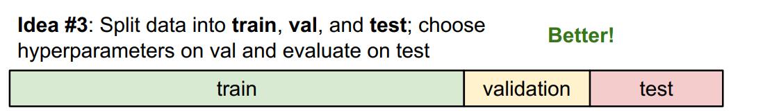
确定方式:将数据集分成训练集、验证集、测试集。通过验证集尝试调整不同超参数,最后在测试集上评估。
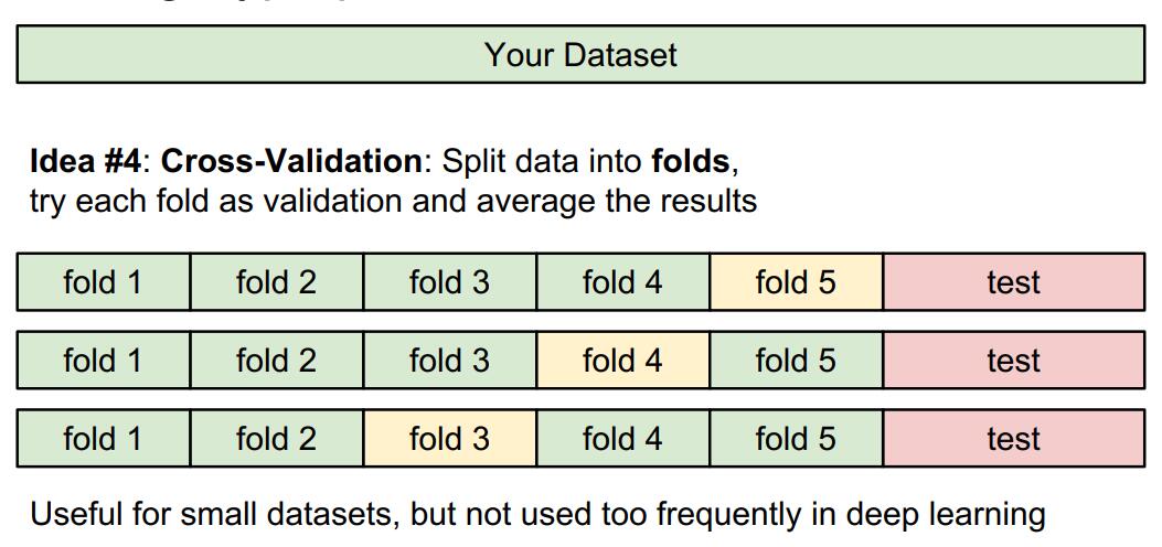
交叉验证方式:将数据集分成5份,其中4份用来训练,其中1份用来验证,并且循环利用每份作为验证集。
代码实现
读入数据
# Load the raw CIFAR-10 data.
cifar10_dir = 'cs231n/datasets/cifar-10-batches-py'

# Cleaning up variables to prevent loading data multiple times (which may cause memory issue)
try:
   del X_train, y_train
   del X_test, y_test
   print('Clear previously loaded data.')
except:
   pass

X_train, y_train, X_test, y_test = load_CIFAR10(cifar10_dir)

# As a sanity check, we print out the size of the training and test data.
print('Training data shape: ', X_train.shape)
print('Training labels shape: ', y_train.shape)
print('Test data shape: ', X_test.shape)
print('Test labels shape: ', y_test.shape)
Training data shape: (50000, 32, 32, 3)
Training labels shape: (50000,)
Test data shape: (10000, 32, 32, 3)
Test labels shape: (10000,)
可以发现每张图片是三信道32*32的矩阵。
可视化部分图片
# Visualize some examples from the dataset.
# We show a few examples of training images from each class.
classes = ['plane', 'car', 'bird', 'cat', 'deer', 'dog', 'frog', 'horse', 'ship', 'truck']
num_classes = len(classes)
samples_per_class = 7

for y, cls in enumerate(classes):
    idxs = np.flatnonzero(y_train == y)
    idxs = np.random.choice(idxs, samples_per_class, replace=False) # 每类随机选7张图。 "repalce = False"表示不能选相同的
    for i, idx in enumerate(idxs):
        plt_idx = i * num_classes + y + 1 # 在图中的位置
        plt.subplot(samples_per_class, num_classes, plt_idx) # 把图分成10 * 7个格子
        plt.imshow(X_train[idx].astype('uint8')) # 生成灰度图
        plt.axis('off')
        if i == 0:    # 在每列开头输出类别名
            plt.title(cls)
plt.show()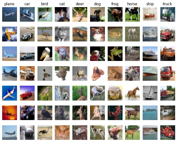
图像数据处理
每张图是32 * 32 * 3的向量不方便处理,我们可以将高维向量变成一维进行存放。
# Subsample the data for more efficient code execution in this exercise
num_training = 5000
mask = list(range(num_training))
X_train = X_train[mask]
y_train = y_train[mask]

num_test = 500
mask = list(range(num_test))
X_test = X_test[mask]
y_test = y_test[mask]
# Reshape the image data into rows
X_train = np.reshape(X_train, (X_train.shape[0], -1))
X_test = np.reshape(X_test, (X_test.shape[0], -1))
print(X_train.shape, X_test.shape)
(5000, 3072) (500, 3072)
操作后训练集变为了5000 * 3072的矩阵,测试集变为了500 * 3072的矩阵。
L2距离的计算
- 使用两层循环:$dist[i][j]$表示第i个测试数据与第j个训练数据的距离。
def compute_distances_two_loops(self, X):
    """
    Compute the distance between each test point in X and each training point
    in self.X_train using a nested loop over both the training data and the
    test data.

    Inputs:
    - X: A numpy array of shape (num_test, D) containing test data.

    Returns:
    - dists: A numpy array of shape (num_test, num_train) where dists[i, j]
      is the Euclidean distance between the ith test point and the jth training
      point.
    """
    num_test = X.shape[0]
    num_train = self.X_train.shape[0]
    dists = np.zeros((num_test, num_train))
    for i in range(num_test):
        for j in range(num_train):
            # *****START OF YOUR CODE (DO NOT DELETE/MODIFY THIS LINE)*****
            dists[i][j] = np.sqrt(np.sum(np.square(X[i] - self.X_train[j])))
            # *****END OF YOUR CODE (DO NOT DELETE/MODIFY THIS LINE)*****
    return dists
使用一层循环:使用numpy函数少写一层循环(但复杂度没变)
def compute_distances_one_loop(self, X):
     """
     Compute the distance between each test point in X and each training point
     in self.X_train using a single loop over the test data.

     Input / Output: Same as compute_distances_two_loops
     """
     num_test = X.shape[0]
     num_train = self.X_train.shape[0]
     dists = np.zeros((num_test, num_train))
     for i in range(num_test):
         # *****START OF YOUR CODE (DO NOT DELETE/MODIFY THIS LINE)*****
         dists[i] = np.sqrt(np.sum(np.square(X[i] - self.X_train), axis = 1))
         # *****END OF YOUR CODE (DO NOT DELETE/MODIFY THIS LINE)*****
     return dists
不使用循环
用A表示第i个测试矩阵$(N\times L)$,B表示第j个训练矩阵$(M \times L)$。根据距离公式:
$$
\begin{aligned}
d_2(i, j) =& \sqrt{\sum_k (A_{ik} - B_{jk})^2}\
=& \sqrt{\sum_k (A_{ik}^2 + B_{jk}^2 - 2 A_{ik}\cdot B_{jk})}\
=& \sqrt{\sum_k A_{ik}^2 + \sum_k B_{jk}^2 - 2(A\cdot B’)_{ij}}
\end{aligned}
$$
$dist[i][j]$表示测试矩阵第i行每个数依次减去训练矩阵第j行每个数后,再平方求和。我们将平方差展开,$dist[i][j]$则可以表示矩阵A第i行每个数平方的和,加上矩阵B第j行每个数平方的和,减去矩阵A与矩阵B转置矩乘后第i行j列的值。
def compute_distances_no_loops(self, X):
    """
    Compute the distance between each test point in X and each training point
    in self.X_train using no explicit loops.

    Input / Output: Same as compute_distances_two_loops
    """
    num_test = X.shape[0]
    num_train = self.X_train.shape[0]
    dists = np.zeros((num_test, num_train))
    # *****START OF YOUR CODE (DO NOT DELETE/MODIFY THIS LINE)*****
    ab = np.dot(X, self.X_train.T)
    a2 = np.sum(np.square(X), axis=1).reshape(-1, 1)
    b2 = np.sum(np.square(self.X_train), axis = 1).reshape(1, -1)
    dists = np.sqrt(a2 + b2 - 2 * ab)
    # *****END OF YOUR CODE (DO NOT DELETE/MODIFY THIS LINE)*****
    return dists
比较三种写法的计算时间
# Let's compare how fast the implementations are
def time_function(f, *args):
    """
    Call a function f with args and return the time (in seconds) that it took to execute.
    """
    import time
    tic = time.time()
    f(*args)
    toc = time.time()
    return toc - tic

two_loop_time = time_function(classifier.compute_distances_two_loops, X_test)
print('Two loop version took %f seconds' % two_loop_time)

one_loop_time = time_function(classifier.compute_distances_one_loop, X_test)
print('One loop version took %f seconds' % one_loop_time)

no_loop_time = time_function(classifier.compute_distances_no_loops, X_test)
print('No loop version took %f seconds' % no_loop_time)

# You should see significantly faster performance with the fully vectorized implementation!

# NOTE: depending on what machine you're using,
# you might not see a speedup when you go from two loops to one loop,
# and might even see a slow-down.
Two loop version took 41.231337 seconds
One loop version took 44.618606 seconds
No loop version took 0.619477 seconds
可以发现不用循环计算速度较前两种快了很多,分析复杂度:
假设测试数据为N,训练数据M,维度为L=3072。
暴力枚举:$O(NML^2)$。
使用矩阵乘法加速后:$O(NML)$。
可视化距离矩阵
plt.imshow(dists, interpolation='none')
plt.show()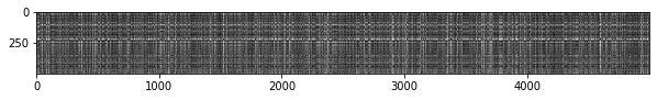
Inline Question 1
Notice the structured patterns in the distance matrix, where some rows or columns are visibly brighter. (Note that with the default color scheme black indicates low distances while white indicates high distances.)
- What in the data is the cause behind the distinctly bright rows?
- What causes the columns?
$\color{blue}{\textit Your Answer:}$
- 导致某些行很亮的原因:若第$i$行很亮,则说明第$i$个测试数据与多数训练数据差异都很大,可能大部分训练数据都没有出现第$i$个测试数据对应的类别。
- 导致某些列很亮的原因:若第$j$列很亮,则说明第$j$个训练数据与多数测试数据差异很大,可能该训练数据对应的类别很少在测试数据集中出现。
标签预测
def predict_labels(self, dists, k=1):
        """
        Given a matrix of distances between test points and training points,
        predict a label for each test point.

        Inputs:
        - dists: A numpy array of shape (num_test, num_train) where dists[i, j]
          gives the distance betwen the ith test point and the jth training point.

        Returns:
        - y: A numpy array of shape (num_test,) containing predicted labels for the
          test data, where y[i] is the predicted label for the test point X[i].
        """
        num_test = dists.shape[0]
        y_pred = np.zeros(num_test)
        for i in range(num_test):
            # A list of length k storing the labels of the k nearest neighbors to
            # the ith test point.
            closest_y = []
            # *****START OF YOUR CODE (DO NOT DELETE/MODIFY THIS LINE)*****
            k_idxs = np.argsort(dists[i])[0: k]
            closest_y = self.y_train[k_idxs]

            # *****END OF YOUR CODE (DO NOT DELETE/MODIFY THIS LINE)*****
            # *****START OF YOUR CODE (DO NOT DELETE/MODIFY THIS LINE)*****
            counts = np.bincount(closest_y)
            y_pred[i] = np.argmax(counts)

            # *****END OF YOUR CODE (DO NOT DELETE/MODIFY THIS LINE)*****

        return y_pred
正确率计算
测试k=1时的结果:
# Now implement the function predict_labels and run the code below:
# We use k = 1 (which is Nearest Neighbor).
y_test_pred = classifier.predict_labels(dists, k=1)

# Compute and print the fraction of correctly predicted examples
num_correct = np.sum(y_test_pred == y_test)
accuracy = float(num_correct) / num_test
print('Got %d / %d correct => accuracy: %f' % (num_correct, num_test, accuracy))
Got 137 / 500 correct => accuracy: 0.274000
测试k=5时的结果:
y_test_pred = classifier.predict_labels(dists, k=5)
num_correct = np.sum(y_test_pred == y_test)
accuracy = float(num_correct) / num_test
print('Got %d / %d correct => accuracy: %f' % (num_correct, num_test, accuracy))
Got 139 / 500 correct => accuracy: 0.278000
Inline Question 2
We can also use other distance metrics such as L1 distance.
For pixel values $p_{ij}^{(k)}$ at location $(i,j)$ of some image $I_k$,
the mean $\mu$ across all pixels over all images is $$\mu=\frac{1}{nhw}\sum_{k=1}^n\sum_{i=1}^{h}\sum_{j=1}^{w}p_{ij}^{(k)}$$
And the pixel-wise mean $\mu_{ij}$ across all images is
$$\mu_{ij}=\frac{1}{n}\sum_{k=1}^np_{ij}^{(k)}.$$
The general standard deviation $\sigma$ and pixel-wise standard deviation $\sigma_{ij}$ is defined similarly.
Which of the following preprocessing steps will not change the performance of a Nearest Neighbor classifier that uses L1 distance? Select all that apply.
- Subtracting the mean $\mu$ ($\tilde{p}{ij}^{(k)}=p{ij}^{(k)}-\mu$.)
- Subtracting the per pixel mean $\mu_{ij}$ ($\tilde{p}{ij}^{(k)}=p{ij}^{(k)}-\mu_{ij}$.)
- Subtracting the mean $\mu$ and dividing by the standard deviation $\sigma$.
- Subtracting the pixel-wise mean $\mu_{ij}$ and dividing by the pixel-wise standard deviation $\sigma_{ij}$.
- Rotating the coordinate axes of the data.
$\color{blue}{\textit Your Answer:}$1, 2, 3
$\color{blue}{\textit Your Explanation:}$
- 每个像素值减一个相同的数,计算L1作差时会被消除,L1的值不会改变
- 对应位置相同的像素点减去一个相同的数,计算L1是对应位置相减,L1的值不会改变
- 每个像素值除以一个相同的值,相当于原L1的值除以$\sigma$,虽然L1的值发生了改变,但是不会影响分类器的效果。
- 不同位置的像素值除以一个不同的值,相当于不同位置有一个不同的权值,导致部分位置的影响增大或减小,会改变L1的值,可能会影响分类器的效果。但是题目中提到$\sigma_{ij}$与$\sigma$可视为相似,在这个条件大概率不会影响。
- L1的值跟坐标系选取有关,旋转坐标系后会影响效果。
交叉验证
num_folds = 5
k_choices = [1, 3, 5, 8, 10, 12, 15, 20, 50, 100]

X_train_folds = []
y_train_folds = []
# *****START OF YOUR CODE (DO NOT DELETE/MODIFY THIS LINE)*****
X_train_folds = np.array_split(X_train, num_folds, axis=0)
y_train_folds = np.array_split(y_train, num_folds, axis=0)
# *****END OF YOUR CODE (DO NOT DELETE/MODIFY THIS LINE)*****
# A dictionary holding the accuracies for different values of k that we find
# when running cross-validation. After running cross-validation,
# k_to_accuracies[k] should be a list of length num_folds giving the different
# accuracy values that we found when using that value of k.
k_to_accuracies = {}
# *****START OF YOUR CODE (DO NOT DELETE/MODIFY THIS LINE)*****
for k in k_choices:
  accuracies = []
  for i in range(num_folds):
    X_train_cross = np.vstack(X_train_folds[: i] + X_train_folds[i + 1 :])
    y_train_cross = np.hstack(y_train_folds[: i] + y_train_folds[i + 1:])
    classifier.train(X_train_cross, y_train_cross)

    X_test_cross = X_train_folds[i]
    y_test_cross = y_train_folds[i]
    y_test_pred = classifier.predict(X_test_cross, k, 0)

    num_correct = np.sum(y_test_pred == y_test_cross)
    accuracies.append(float(num_correct) / X_test_cross.shape[0])
  k_to_accuracies[k] = accuracies
# *****END OF YOUR CODE (DO NOT DELETE/MODIFY THIS LINE)*****

# Print out the computed accuracies
for k in sorted(k_to_accuracies):
    for accuracy in k_to_accuracies[k]:
        print('k = %d, accuracy = %f' % (k, accuracy))
k = 1, accuracy = 0.263000
k = 1, accuracy = 0.257000
k = 1, accuracy = 0.264000
…
k = 100, accuracy = 0.270000
k = 100, accuracy = 0.263000
k = 100, accuracy = 0.256000
k = 100, accuracy = 0.263000
可视化选取k值
# plot the raw observations
for k in k_choices:
    accuracies = k_to_accuracies[k]
    plt.scatter([k] * len(accuracies), accuracies)

# plot the trend line with error bars that correspond to standard deviation
accuracies_mean = np.array([np.mean(v) for k,v in sorted(k_to_accuracies.items())])
accuracies_std = np.array([np.std(v) for k,v in sorted(k_to_accuracies.items())])
plt.errorbar(k_choices, accuracies_mean, yerr=accuracies_std)
plt.title('Cross-validation on k')
plt.xlabel('k')
plt.ylabel('Cross-validation accuracy')
plt.show()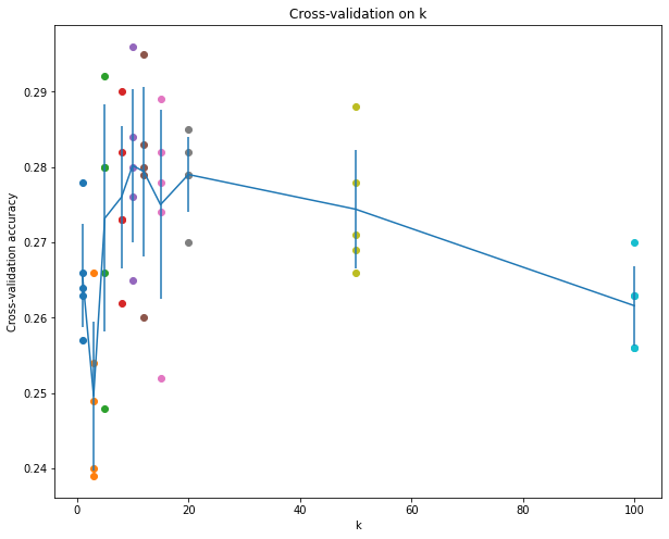
根据图像观察,当k值为10左右,效果较好:
# Based on the cross-validation results above, choose the best value for k,
# retrain the classifier using all the training data, and test it on the test
# data. You should be able to get above 28% accuracy on the test data.
best_k = 10

classifier = KNearestNeighbor()
classifier.train(X_train, y_train)
y_test_pred = classifier.predict(X_test, k=best_k)

# Compute and display the accuracy
num_correct = np.sum(y_test_pred == y_test)
accuracy = float(num_correct) / num_test
print('Got %d / %d correct => accuracy: %f' % (num_correct, num_test, accuracy))
Got 141 / 500 correct => accuracy: 0.282000
Inline Question 3
Which of the following statements about $k$-Nearest Neighbor ($k$-NN) are true in a classification setting, and for all $k$? Select all that apply.
- The decision boundary of the k-NN classifier is linear.
- The training error of a 1-NN will always be lower than or equal to that of 5-NN.
- The test error of a 1-NN will always be lower than that of a 5-NN.
- The time needed to classify a test example with the k-NN classifier grows with the size of the training set.
- None of the above.
$\color{blue}{\textit Your Answer:}$ 2, 4
$\color{blue}{\textit Your Explanation:}$
- knn根据周围最近邻的k个点投票决定,这个思想无法保证决策边界一定是线性的。
- 1-NN表示只有最近邻点作为依据,是没有训练误差的。
- k越小,测试误差越大。
- 每次test都要与训练数据矩阵做矩乘,训练集越大,花费时间越长。
KNN总结
优点
- 算法容易理解,思路简单
- 分类器训练时间短
- 适用于各种分类问题
缺点
代码实现的KNN分类器最优的结果也只有28.2%的正确率,正确率太低
训练$O(1)$,测试$O(n)$。预测时间与训练集大小正相关,预测不方便
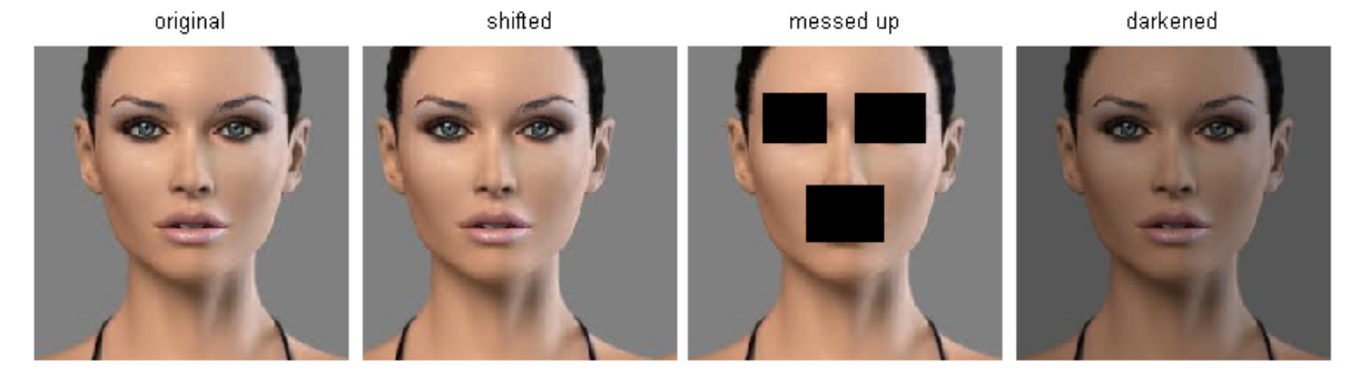
暴力采用像素点距离差异作为判别依据十分不准确,容易分辨错误。例如下图,后三张不同的图片到第一张图的L2相同。