Task
使用KNN进行Iris 鸢尾花分类
导入模块
import pandas as pd
import numpy as np
import matplotlib.pyplot as plt
import seaborn as sns

from sklearn.neighbors import KNeighborsClassifier
from sklearn.metrics import accuracy_score

plt.rcParams['font.sans-serif'] = ['Microsoft YaHei']
%matplotlib inline
查看数据
# 读取数据
feat_names = ['sepal-length', 'sepal-width', 'petal-length', 'petal-width', 'species']
dpath = '../data/'
df = pd.read_csv(dpath + 'iris.csv', names=feat_names)

df.head()| sepal-length | sepal-width | petal-length | petal-width | species | |
|---|---|---|---|---|---|
| 0 | 5.1 | 3.5 | 1.4 | 0.2 | Iris-setosa |
| 1 | 4.9 | 3.0 | 1.4 | 0.2 | Iris-setosa |
| 2 | 4.7 | 3.2 | 1.3 | 0.2 | Iris-setosa |
| 3 | 4.6 | 3.1 | 1.5 | 0.2 | Iris-setosa |
| 4 | 5.0 | 3.6 | 1.4 | 0.2 | Iris-setosa |
# 查看数据总体情况
df.info()
<class 'pandas.core.frame.DataFrame'>
RangeIndex: 150 entries, 0 to 149
Data columns (total 5 columns):
# Column Non-Null Count Dtype
--- ------ -------------- -----
0 sepal-length 150 non-null float64
1 sepal-width 150 non-null float64
2 petal-length 150 non-null float64
3 petal-width 150 non-null float64
4 species 150 non-null object
dtypes: float64(4), object(1)
memory usage: 6.0+ KB
# 查看缺失值情况
column_null = df.isnull().sum(axis=0)
row_null = df.isnull().sum(axis=1)
all_null = df.isnull().sum().sum()
all_null
0
# 查看数值型特征的统计量
df.describe()| sepal-length | sepal-width | petal-length | petal-width | |
|---|---|---|---|---|
| count | 150.000000 | 150.000000 | 150.000000 | 150.000000 |
| mean | 5.843333 | 3.054000 | 3.758667 | 1.198667 |
| std | 0.828066 | 0.433594 | 1.764420 | 0.763161 |
| min | 4.300000 | 2.000000 | 1.000000 | 0.100000 |
| 25% | 5.100000 | 2.800000 | 1.600000 | 0.300000 |
| 50% | 5.800000 | 3.000000 | 4.350000 | 1.300000 |
| 75% | 6.400000 | 3.300000 | 5.100000 | 1.800000 |
| max | 7.900000 | 4.400000 | 6.900000 | 2.500000 |
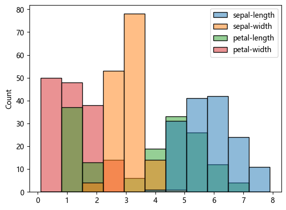
# 特征的直方图
sns.histplot(df)
<Axes: ylabel='Count'>
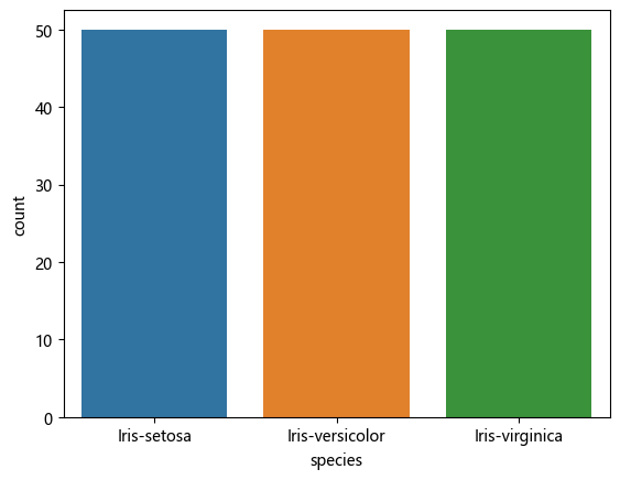
# 标签的直方图
sns.countplot(df, x = 'species')
<Axes: xlabel='species', ylabel='count'>
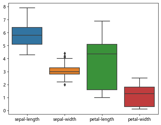
# IQR 检测噪声
sns.boxplot(df)
<Axes: >
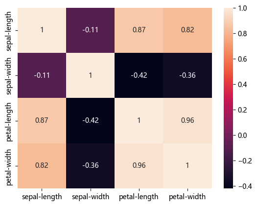
# 查看数值型特征之间的相关系数
feat_corr = df.select_dtypes(include=['number']).corr()
sns.heatmap(feat_corr, annot=True)
<Axes: >
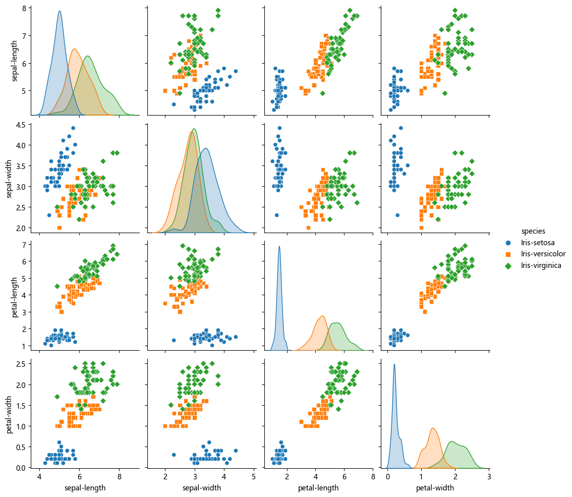
# 查看特征两两之间的散点图
sns.pairplot(df, hue='species', kind='scatter', diag_kind='kde', markers=["o", "s", "D"], diag_kws=dict(fill=True))
d:\Anaconda3\Lib\site-packages\seaborn\axisgrid.py:118: UserWarning: The figure layout has changed to tight
self._figure.tight_layout(*args, **kwargs)
<seaborn.axisgrid.PairGrid at 0x1e63c538c50>
数据预处理
# 将标签字符串映射为整数
target_map = {'Iris-setosa':0,
              'Iris-versicolor':1,
              'Iris-virginica':2 }

df['species'] = df['species'].apply(lambda x: target_map[x])
df.head()| sepal-length | sepal-width | petal-length | petal-width | species | |
|---|---|---|---|---|---|
| 0 | 5.1 | 3.5 | 1.4 | 0.2 | 0 |
| 1 | 4.9 | 3.0 | 1.4 | 0.2 | 0 |
| 2 | 4.7 | 3.2 | 1.3 | 0.2 | 0 |
| 3 | 4.6 | 3.1 | 1.5 | 0.2 | 0 |
| 4 | 5.0 | 3.6 | 1.4 | 0.2 | 0 |
# 从原始数据分离x, y
y = df['species']
X = df.drop('species', axis=1)
X, y
( sepal-length sepal-width petal-length petal-width
0 5.1 3.5 1.4 0.2
1 4.9 3.0 1.4 0.2
2 4.7 3.2 1.3 0.2
3 4.6 3.1 1.5 0.2
4 5.0 3.6 1.4 0.2
.. ... ... ... ...
145 6.7 3.0 5.2 2.3
146 6.3 2.5 5.0 1.9
147 6.5 3.0 5.2 2.0
148 6.2 3.4 5.4 2.3
149 5.9 3.0 5.1 1.8
[150 rows x 4 columns],
0 0
1 0
2 0
3 0
4 0
..
145 2
146 2
147 2
148 2
149 2
Name: species, Length: 150, dtype: int64)
# 特征缩放
from sklearn.preprocessing import StandardScaler

scaler = StandardScaler()
scaler.fit(X)

X = scaler.transform(X)plt.scatter(df['petal-length'], df['petal-width'], label='origin')
plt.scatter(X[:, 2], X[:, 3], label = 'standerlized')
x_ticks = np.arange(-2, 8, 1)
plt.xticks(x_ticks)
plt.yticks(x_ticks)
plt.xlabel('petal-length')
plt.ylabel('petal-width')
plt.legend()
plt.show()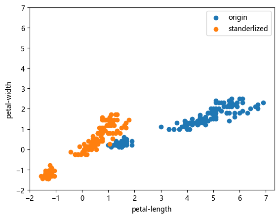
# 数据划分
from sklearn.model_selection import train_test_split

X_train, X_test, y_train, y_test = train_test_split(X, y, test_size=0.2, random_state=42, stratify=y)
模型训练
# 5折交叉验证初步测试,大致确定参数范围
from sklearn.model_selection import cross_val_score

knn = KNeighborsClassifier(n_neighbors=31)
scores = cross_val_score(knn, X_train, y_train)
print("Cross-validation scores: {}".format(scores))
print("Average cross-validation score: {:.2f}".format(scores.mean()))
Cross-validation scores: [0.875 0.91666667 0.83333333 0.91666667 0.91666667]
Average cross-validation score: 0.89
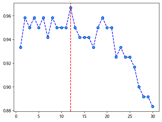
# GridSearch参数搜索
from sklearn.model_selection import GridSearchCV

Ks = range(1, 31)
tuned_parameters = dict(n_neighbors=Ks)
knn = KNeighborsClassifier()
grid = GridSearchCV(knn, param_grid=tuned_parameters, cv=10, scoring='accuracy', n_jobs=16, verbose=3)
grid.fit(X_train, y_train)
Fitting 10 folds for each of 30 candidates, totalling 300 fits
# 查找最佳超参数
best_parameter = grid.best_params_['n_neighbors']
best_parameter
12
# 可视化参数搜索结果
accuracy = grid.cv_results_['mean_test_score']
plt.plot(Ks, accuracy, color='b', linestyle='dashed', marker='o', markerfacecolor='c')

plt.axvline(best_parameter, color='r', ls='dashed')
<matplotlib.lines.Line2D at 0x157cc8bf450>
accuracyarray([0.93333333, 0.95833333, 0.95 , 0.95833333, 0.95 ,
0.95833333, 0.94166667, 0.95833333, 0.95 , 0.95 ,
0.95 , 0.96666667, 0.95 , 0.94166667, 0.94166667,
0.94166667, 0.93333333, 0.95 , 0.95833333, 0.95 ,
0.95 , 0.925 , 0.93333333, 0.925 , 0.925 ,
0.91666667, 0.9 , 0.89166667, 0.89166667, 0.88333333])
accuracy[best_parameter-1]0.9666666666666666
# 在测试集上测试
y_test_pred = grid.predict(X_test)
acc = accuracy_score(y_test, y_test_pred)
acc
0.9666666666666667
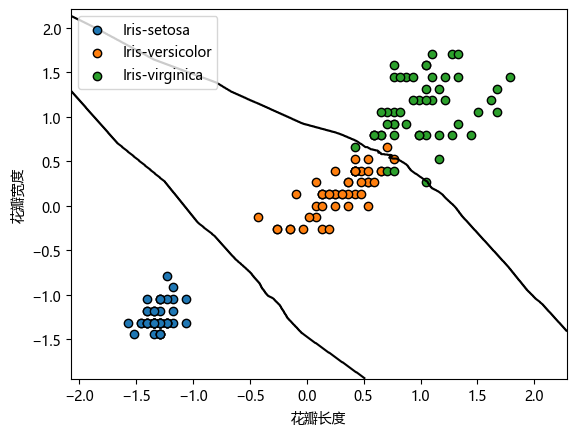
取后两维特征,在2D平面上可视化决策边界
# 用最佳超参数在所有训练数据上训练
X_train = X
y_train = y

X_train_2d = X[:, 2:]
knn = KNeighborsClassifier(n_neighbors=12)
knn.fit(X_train_2d, y_train)
y_predict = knn.predict(X_test[:, 2:])
accuracy_score(y_predict, y_test)0.9333333333333333
knn.predict_proba([[-0.5, -1.5], [0.01, 0.9], [-0.1, -0.32], [0.9, -0.45]])array([[1. , 0. , 0. ],
[0. , 0.58333333, 0.41666667],
[0. , 1. , 0. ],
[0. , 0.91666667, 0.08333333]])
# 函数:画出分类器决策边界
def plot_2d_separator(classifier, X, eps=None):
    if eps is None:
        eps = X.std() / 2
    x1_min, x2_min = X.min(axis=0) - eps
    x1_max, x2_max = X.max(axis=0) + eps
    x1 = np.linspace(x1_min, x1_max, 1000)
    x2 = np.linspace(x2_min, x2_max, 1000)

    X1, X2 = np.meshgrid(x1, x2)
    X_grid = np.c_[X1.ravel(), X2.ravel()]

    decision_values = classifier.predict_proba(X_grid)[:, 1]
    levels = [.5]

    ax = plt.gca()
    ax.contour(X1, X2, decision_values.reshape(X1.shape), levels=levels, colors="black")

    ax.set_xlim(x1_min, x1_max)
    ax.set_ylim(x2_min, x2_max)
    # ax.set_xticks(())
    # ax.set_yticks(())
# 可视化结果
import matplotlib as mpl

color = ['tab:blue', 'tab:orange', 'tab:green']

target_map = {0: 'Iris-setosa',
              1: 'Iris-versicolor',
              2: 'Iris-virginica'}
for i in range(3):
    X_i = X_train_2d[y_train==i]
    scatter = plt.scatter(X_i[:, 0], X_i[:, 1], c=color[i], marker='o', edgecolors='k', label=target_map[i])
plot_2d_separator(knn, X_train_2d)

plt.xlabel('花瓣长度')
plt.ylabel('花瓣宽度')
plt.legend()
plt.show()