使用朴素贝叶斯和高斯判别分析进行Iris分类

Task

使用朴素贝叶斯模型和高斯判别分析模型对iris分类

导入模块

import numpy as np
import pandas as pd
import matplotlib.pyplot as plt
import seaborn as sns

from sklearn.metrics import accuracy_score 
plt.rcParams['font.sans-serif'] = ['Microsoft YaHei']
%matplotlib inline

查看数据

# 读取数据
feat_names = ['sepal-length', 'sepal-width', 'petal-length', 'petal-width', 'species']
dpath = '../data/'
df = pd.read_csv(dpath + 'iris.csv', names=feat_names)

df.head()

	sepal-length	sepal-width	petal-length	petal-width	species
0	5.1	3.5	1.4	0.2	Iris-setosa
1	4.9	3.0	1.4	0.2	Iris-setosa
2	4.7	3.2	1.3	0.2	Iris-setosa
3	4.6	3.1	1.5	0.2	Iris-setosa
4	5.0	3.6	1.4	0.2	Iris-setosa

# 查看数据总体情况
df.info()

<class 'pandas.core.frame.DataFrame'>
RangeIndex: 150 entries, 0 to 149
Data columns (total 5 columns):
 #   Column        Non-Null Count  Dtype  
---  ------        --------------  -----  
 0   sepal-length  150 non-null    float64
 1   sepal-width   150 non-null    float64
 2   petal-length  150 non-null    float64
 3   petal-width   150 non-null    float64
 4   species       150 non-null    object 
dtypes: float64(4), object(1)
memory usage: 6.0+ KB

# 查看缺失值情况
column_null = df.isnull().sum(axis=0)
row_null = df.isnull().sum(axis=1)
all_null = df.isnull().sum().sum()
all_null

0

# 查看数值型特征的统计量
df.describe()

	sepal-length	sepal-width	petal-length	petal-width
count	150.000000	150.000000	150.000000	150.000000
mean	5.843333	3.054000	3.758667	1.198667
std	0.828066	0.433594	1.764420	0.763161
min	4.300000	2.000000	1.000000	0.100000
25%	5.100000	2.800000	1.600000	0.300000
50%	5.800000	3.000000	4.350000	1.300000
75%	6.400000	3.300000	5.100000	1.800000
max	7.900000	4.400000	6.900000	2.500000

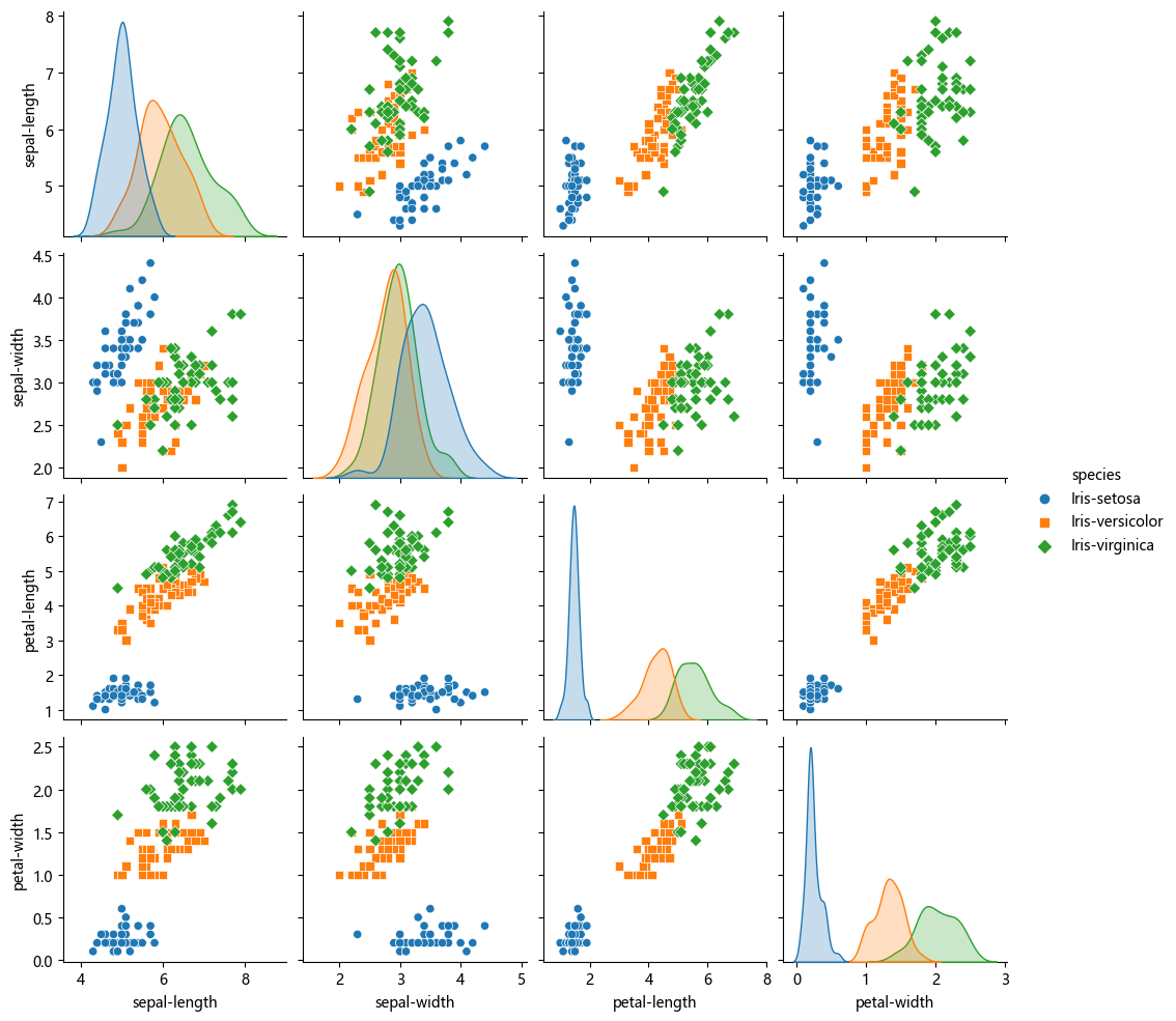
# 查看特征两两之间的散点图
sns.pairplot(df, hue='species', kind='scatter', diag_kind='kde', markers=["o", "s", "D"], diag_kws=dict(fill=True))

d:\Anaconda3\Lib\site-packages\seaborn\axisgrid.py:118: UserWarning: The figure layout has changed to tight
  self._figure.tight_layout(*args, **kwargs)





<seaborn.axisgrid.PairGrid at 0x2f6a5635e10>

数据预处理

# 将标签字符串映射为整数
target_map = {'Iris-setosa':0, 
              'Iris-versicolor':1,
              'Iris-virginica':2 }

df['species'] = df['species'].apply(lambda x: target_map[x])
df.head()

	sepal-length	sepal-width	petal-length	petal-width	species
0	5.1	3.5	1.4	0.2	0
1	4.9	3.0	1.4	0.2	0
2	4.7	3.2	1.3	0.2	0
3	4.6	3.1	1.5	0.2	0
4	5.0	3.6	1.4	0.2	0

# 从原始数据分离x, y
y = df['species']
X = df.drop('species', axis=1)
X, y

(     sepal-length  sepal-width  petal-length  petal-width
 0             5.1          3.5           1.4          0.2
 1             4.9          3.0           1.4          0.2
 2             4.7          3.2           1.3          0.2
 3             4.6          3.1           1.5          0.2
 4             5.0          3.6           1.4          0.2
 ..            ...          ...           ...          ...
 145           6.7          3.0           5.2          2.3
 146           6.3          2.5           5.0          1.9
 147           6.5          3.0           5.2          2.0
 148           6.2          3.4           5.4          2.3
 149           5.9          3.0           5.1          1.8
 
 [150 rows x 4 columns],
 0      0
 1      0
 2      0
 3      0
 4      0
       ..
 145    2
 146    2
 147    2
 148    2
 149    2
 Name: species, Length: 150, dtype: int64)

# 数据划分
from sklearn.model_selection import train_test_split

X_train, X_test, y_train, y_test = train_test_split(X, y, test_size=0.2, random_state=42, stratify=y)

模型训练

朴素贝叶斯模型

朴素贝叶斯模型： https://scikit-learn.org/stable/modules/naive_bayes.html#gaussian-naive-bayes

贝叶斯公式: $P(y|x) = \frac{P(xy)}{P(x)} = \frac{P(x|y)P(y)}{P(x)}$

朴素贝叶斯模型就是根据贝叶斯公式进行设计，inference时对于给定的输入x，将x作为条件，判断每一个标签y的概率。这是一种非常简单而且自然的想法，我们拿到一堆数据去预测另一个未知输入时，不就是在已有的数据里寻找输入和输出之间的潜在规律，然后按照这个规律去看新的输入最大可能的输出是多少。所以训练的目标很简单，就是让预测的概率尽可能地正确。

首先看分母，对于一个输入x，$P(x)$是一个定值，可以不用管。我们只需要把$P(y)$和$P(x|y)$预测好就行了。$P(y)$称为类先验分布，通俗地说是每个类出现的几率。$P(X|y)$称为类条件概率，即在确定类别的条件下，出现这个x的概率。为了估算这两个值，我们需要假设y, x|y服从的分布情况。一般常用的分布有高斯分布、Multinoulli分布等。

值得注意的是，朴素贝叶斯模型假设各个特征之间是相互独立的，这个假设大大简化了模型。尽管这个假设非常强，但在现实世界中朴素贝叶斯模型在很多情况下还是有不错的效果。

from sklearn.naive_bayes import GaussianNB


gnb = GaussianNB()
gnb.fit(X_train, y_train)
y_train_pred = gnb.predict(X_train)
y_test_pred = gnb.predict(X_test)
print('train loss: {}'.format(accuracy_score(y_train_pred, y_train)))
print('test loss: {}'.format(accuracy_score(y_test_pred, y_test)))

train loss: 0.9583333333333334
test loss: 0.9666666666666667

print('预测类别: ',gnb.classes_)
print('类先验概率: ',gnb.class_prior_)
print('均值: ', gnb.theta_)
print('方差: ', gnb.var_)

预测类别:  [0 1 2]
类先验概率:  [0.33333333 0.33333333 0.33333333]
均值:  [[4.985  3.4025 1.48   0.2525]
 [5.93   2.75   4.2525 1.32  ]
 [6.61   2.98   5.58   2.04  ]]
方差:  [[0.092775   0.15674375 0.0251     0.01349375]
 [0.2216     0.093      0.19149375 0.0341    ]
 [0.4574     0.1221     0.3236     0.0704    ]]

二次判别分析 Quadratic Discriminant Analysis

二次判别分析：https://scikit-learn.org/stable/modules/lda_qda.html

朴素贝叶斯模型认为各个特征相互独立，二次判别分析则使用多元高斯分布去刻画这些特征分布。

也就是说朴素贝叶斯模型是二次判别分析一种特殊情况。

朴素贝叶斯模型 = QDA + 特征之间独立

LDA = QDA + QDA + 不同类别特征的协方差相同

from sklearn.discriminant_analysis import QuadraticDiscriminantAnalysis

qda = QuadraticDiscriminantAnalysis(store_covariance=True)
qda.fit(X_train, y_train)
y_train_pred = qda.predict(X_train)
y_test_pred = qda.predict(X_test)
print('train loss: {}'.format(accuracy_score(y_train_pred, y_train)))
print('test loss: {}'.format(accuracy_score(y_test_pred, y_test)))

train loss: 0.975
test loss: 1.0

print('类先验：')
print(qda.priors_ )                   

print('均值：')
print(qda.means_)                           

print('协方差矩阵：')
print(qda.covariance_)

print('主轴方向：')
print(qda.rotations_)

print("主轴方向的方差:")
print(qda.scalings_)

类先验：
[0.33333333 0.33333333 0.33333333]
均值：
[[4.985  3.4025 1.48   0.2525]
 [5.93   2.75   4.2525 1.32  ]
 [6.61   2.98   5.58   2.04  ]]
协方差矩阵：
[array([[0.09515385, 0.09644872, 0.0094359 , 0.01260256],
       [0.09644872, 0.16076282, 0.01569231, 0.01422436],
       [0.0094359 , 0.01569231, 0.02574359, 0.00569231],
       [0.01260256, 0.01422436, 0.00569231, 0.01383974]]), array([[0.22728205, 0.06538462, 0.14992308, 0.04092308],
       [0.06538462, 0.09538462, 0.06269231, 0.03358974],
       [0.14992308, 0.06269231, 0.19640385, 0.06046154],
       [0.04092308, 0.03358974, 0.06046154, 0.03497436]]), array([[0.46912821, 0.11302564, 0.35123077, 0.04882051],
       [0.11302564, 0.12523077, 0.09394872, 0.05235897],
       [0.35123077, 0.09394872, 0.33189744, 0.05876923],
       [0.04882051, 0.05235897, 0.05876923, 0.07220513]])]
主轴方向：
[array([[ 0.577788  ,  0.73618305, -0.31761196, -0.1527029 ],
       [ 0.80647248, -0.47185993,  0.35401286,  0.04031434],
       [ 0.08971131, -0.48493266, -0.81656606, -0.3000201 ],
       [ 0.08783536, -0.01493412, -0.32713515,  0.94076805]]), array([[-0.68454964,  0.60008382, -0.39870293, -0.11102777],
       [-0.29380636, -0.70158636, -0.61189706,  0.21687874],
       [-0.63479501, -0.22071006,  0.66978334,  0.31577309],
       [-0.20519479, -0.31458393,  0.13419481, -0.91701897]]), array([[ 0.74623282, -0.2620598 ,  0.43418988,  0.43120806],
       [ 0.21974119,  0.7874671 ,  0.45198579, -0.35681678],
       [ 0.61764038, -0.06722203, -0.59012686, -0.51551125],
       [ 0.11563196,  0.5538063 , -0.50885979,  0.64883707]])]
主轴方向的方差:
[array([0.23315722, 0.0268634 , 0.02489103, 0.01058835]), array([0.40663798, 0.07424305, 0.06199862, 0.01116522]), array([0.80068144, 0.11642003, 0.05219651, 0.02916357])]

# 带缩放的QDA 
# Regularizes the per-class covariance estimates by transforming S2 as S2 = (1 - reg_param) * S2 + reg_param * np.eye(n_features)

qda = QuadraticDiscriminantAnalysis(reg_param=0.1, store_covariance=True)
qda.fit(X_train, y_train)
y_train_pred = qda.predict(X_train)
y_test_pred = qda.predict(X_test)
print('train loss: {}'.format(accuracy_score(y_train_pred, y_train)))
print('test loss: {}'.format(accuracy_score(y_test_pred, y_test)))

train loss: 0.975
test loss: 0.9666666666666667