Task
使用Fisher判别分析对iris进行降维与分类
导入模块
import numpy as np
import pandas as pd
import matplotlib.pyplot as plt
import seaborn as sns

from sklearn.metrics import accuracy_score
plt.rcParams['font.sans-serif'] = ['Microsoft YaHei']
%matplotlib inline
查看数据
# 读取数据(数据的检查可见“使用KNN进行Iris分类使用KNN进行Iris分类”一节,此处省略)
feat_names = ['sepal-length', 'sepal-width', 'petal-length', 'petal-width', 'species']
dpath = '../data/'
df = pd.read_csv(dpath + 'iris.csv', names=feat_names)

df.head()| sepal-length | sepal-width | petal-length | petal-width | species | |
|---|---|---|---|---|---|
| 0 | 5.1 | 3.5 | 1.4 | 0.2 | Iris-setosa |
| 1 | 4.9 | 3.0 | 1.4 | 0.2 | Iris-setosa |
| 2 | 4.7 | 3.2 | 1.3 | 0.2 | Iris-setosa |
| 3 | 4.6 | 3.1 | 1.5 | 0.2 | Iris-setosa |
| 4 | 5.0 | 3.6 | 1.4 | 0.2 | Iris-setosa |
数据预处理
# 将标签字符串映射为整数
target_map = {'Iris-setosa':0,
              'Iris-versicolor':1,
              'Iris-virginica':2 }

df['species'] = df['species'].apply(lambda x: target_map[x])
df.head()| sepal-length | sepal-width | petal-length | petal-width | species | |
|---|---|---|---|---|---|
| 0 | 5.1 | 3.5 | 1.4 | 0.2 | 0 |
| 1 | 4.9 | 3.0 | 1.4 | 0.2 | 0 |
| 2 | 4.7 | 3.2 | 1.3 | 0.2 | 0 |
| 3 | 4.6 | 3.1 | 1.5 | 0.2 | 0 |
| 4 | 5.0 | 3.6 | 1.4 | 0.2 | 0 |
# 从原始数据分离x, y
y = df['species']
X = df.drop('species', axis=1)
X, y
( sepal-length sepal-width petal-length petal-width
0 5.1 3.5 1.4 0.2
1 4.9 3.0 1.4 0.2
2 4.7 3.2 1.3 0.2
3 4.6 3.1 1.5 0.2
4 5.0 3.6 1.4 0.2
.. ... ... ... ...
145 6.7 3.0 5.2 2.3
146 6.3 2.5 5.0 1.9
147 6.5 3.0 5.2 2.0
148 6.2 3.4 5.4 2.3
149 5.9 3.0 5.1 1.8
[150 rows x 4 columns],
0 0
1 0
2 0
3 0
4 0
..
145 2
146 2
147 2
148 2
149 2
Name: species, Length: 150, dtype: int64)
# 数据划分
from sklearn.model_selection import train_test_split

X_train, X_test, y_train, y_test = train_test_split(X, y, test_size=0.2, random_state=42, stratify=y)
模型训练
Fisher判别分析是LDA(线性判别分析)中的一种。LDA是希望用一条或多条直线将不同类别的数据进行划分。
在前一章“使用朴素贝叶斯和高斯判别分析进行Iris分类使用朴素贝叶斯和高斯判别分析进行Iris分类”中,从贝叶斯的角度推出了LDA,当时我们提到LDA是QDA+不同类别特征的协方差相同。
而Fisher判别分析是从降维的角度进行推导,设法将数据投影到一条直线上,使得同类数据的投影点尽可能接近,不同类数据的投影点尽可能远离,并提出Fisher 准则函数:
$$ J(W) = \frac{|W^TS_bW|}{|W^TS_wW|}$$
其中,$S_b$为类间散度,$S_w$为类内散度。
通过拉格朗日乘子法,解得最佳投影方向为$w=S_w^{-1}(\mu_1-\mu_2)$
判别函数为$f(x) = w^Tx = (\mu_1-\mu_2)S_w^{-1}x$
在sklearn中,Fisher判别分析调用LinearDiscriminantAnalysis,通过参数n_components控制LDA是作为线性分类器,还是降维。
from sklearn.discriminant_analysis import LinearDiscriminantAnalysis

flda = LinearDiscriminantAnalysis(n_components=2)
X_train_new = flda.fit_transform(X_train, y_train)
print(X_train_new.shape)
plt.scatter(X_train_new[y_train==0,	0],	X_train_new[y_train==0,	1],	marker='o',	c='C4')
plt.scatter(X_train_new[y_train==1,	0],	X_train_new[y_train==1,	1],	marker='o',	c='C0')
plt.scatter(X_train_new[y_train==2,	0],	X_train_new[y_train==2,	1],	marker='o',	c='C1')
plt.legend(target_map.keys(), loc='best', fancybox=True)
plt.show()
(120, 2)
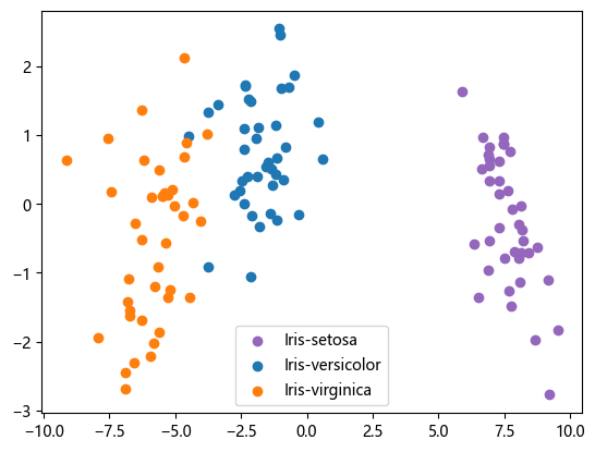
y_pred = flda.predict(X_test)
accuracy_score(y_test, y_pred)
1.0
手动实现
### 观察每个特征在1维的分布
import math
fig, axes = plt.subplots(2, 2)
label = {v: k for k, v in target_map.items()}
for ax, column in zip(axes.ravel(), range(X_train.shape[1])):
    X_column = np.array(X_train[feat_names[column]])

    min_b = math.floor(np.min(X_column))
    max_b = math.ceil(np.max(X_column))
    bins = np.linspace(min_b, max_b, 25)

    for i in range(3):
        ax.hist(X_column[y_train==i], color='C{}'.format(i), label=label[i], bins=bins, alpha=0.5)
    ylims = ax.get_ylim()

    l = ax.legend(loc='upper right', fontsize=8)
    l.get_frame().set_alpha(0.5)
    ax.set_ylim([0, max(ylims) + 2])
    ax.set_title('Iris histogram feature %s' % feat_names[column])

    ax.tick_params(axis='both', which='both', bottom=False, top=False, left=False, right=False,
                   labelbottom=True, labelleft=True)

    ax.spines['top'].set_visible(False)
    ax.spines['right'].set_visible(False)
    ax.spines['bottom'].set_visible(False)
    ax.spines['left'].set_visible(False)

axes[0][0].set_ylabel('count')
axes[1][0].set_ylabel('count')
fig.tight_layout()
plt.show()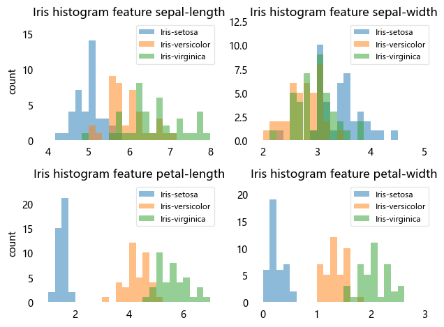
通过以上各个特征的直方图,可以感觉到花瓣的长度和花瓣的宽度更适合分类,而花萼的形状相对更难区分
### 计算每个类别的平均向量

X_train_matrix = np.array(X_train)
mean_vector = []
for i in range(len(target_map)):
    mean_vector.append(np.mean(X_train_matrix[y_train == i], axis=0))
mean_vector
[array([4.985 , 3.4025, 1.48 , 0.2525]),
array([5.93 , 2.75 , 4.2525, 1.32 ]),
array([6.61, 2.98, 5.58, 2.04])]
### 计算类内散度S_w
S_w = np.zeros((X_train_matrix.shape[1], X_train_matrix.shape[1]))
for i in range(len(target_map)):
    Xi = X_train_matrix[y_train == i] - mean_vector[i]
    S_w += Xi.T @ Xi
print('类内散度:\n', S_w)
类内散度:
[[30.871 10.7195 19.913 3.9915 ]
[10.7195 14.87375 6.721 3.90675]
[19.913 6.721 21.60775 4.872 ]
[ 3.9915 3.90675 4.872 4.71975]]
### 计算类间散度S_b
S_b = np.zeros_like(S_w)

mu = np.mean(X_train_matrix, axis = 0)
for i in range(len(target_map)):
    Ni = len(X_train_matrix[y_train == i])
    mui_mu = (mean_vector[i] - mu).reshape(4, 1)
    S_b += Ni * mui_mu @ mui_mu.T
print('类间散度:\n', S_b)
类间散度:
[[ 53.28066667 -15.29033333 135.80283333 58.70766667]
[-15.29033333 8.76216667 -43.14641667 -17.14883333]
[135.80283333 -43.14641667 350.12016667 149.92258333]
[ 58.70766667 -17.14883333 149.92258333 64.70816667]]
### $w=S_w^{-1}(\mu_1-\mu_2)$是在二分类问题上推出来的,由于不是二分类问题,需要从$\lambda w = S_w^-1S_b w$入手
eigvals, eigvecs = np.linalg.eig(np.linalg.inv(S_w) * S_b)
np.testing.assert_array_almost_equal(np.mat(np.linalg.inv(S_w) * S_b) * np.mat(eigvecs[:, 0].reshape(4, 1)),
                                     eigvals[0] * np.mat(eigvecs[:, 0].reshape(4, 1)), decimal=6, err_msg='',
                                     verbose=True)
# 选择对应特征值最大的两个向量作为降维后的方向
eig_pairs = [(np.abs(eigvals[i]), eigvecs[:, i]) for i in range(len(eigvals))]
eig_pairs = sorted(eig_pairs, key=lambda k: k[0], reverse=True)
W = np.hstack((eig_pairs[0][1].reshape(4, 1), eig_pairs[1][1].reshape(4, 1)))
Warray([[ 0.22158073, 0.14530083],
[ 0.0269259 , -0.05194717],
[-0.90534611, -0.33666352],
[ 0.36128299, -0.92889549]])
X_trans =  X_train_matrix @ W
X_trans.shape
(120, 2)
# 比较手写的LDA与sklearn的LDA

plt.figure(figsize=(8,4))
plt.subplot(121)
plt.scatter(X_trans[y_train==0,	0],	X_trans[y_train==0,	1],	marker='o',	c='C4')
plt.scatter(X_trans[y_train==1,	0],	X_trans[y_train==1,	1],	marker='o',	c='C0')
plt.scatter(X_trans[y_train==2,	0],	X_trans[y_train==2,	1],	marker='o',	c='C1')
plt.title('My LDA')
plt.legend(target_map.keys(), loc='lower right', fancybox=True)

plt.subplot(122)
plt.scatter(X_train_new[y_train==0,	0],	X_train_new[y_train==0,	1],	marker='o',	c='C4')
plt.scatter(X_train_new[y_train==1,	0],	X_train_new[y_train==1,	1],	marker='o',	c='C0')
plt.scatter(X_train_new[y_train==2,	0],	X_train_new[y_train==2,	1],	marker='o',	c='C1')
plt.title('sklearn LDA')
plt.legend(target_map.keys(), loc='lower right', fancybox=True)
plt.show()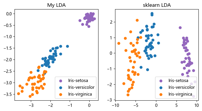
### 多类分类问题,使用一对一分类法,两两类之间建立线性判别函数

def get_Wb_2categories(cat1, cat2):
    mu1 = mean_vector[cat1].reshape(4, 1)
    mu2 = mean_vector[cat2].reshape(4, 1)
    X_1 = X_train_matrix[y_train == cat1] - mean_vector[cat1]
    X_2 = X_train_matrix[y_train == cat2] - mean_vector[cat2]
    S_w_inv = np.linalg.inv(X_1.T @ X_1 + X_2.T @ X_2)
    W_T = (mu1 - mu2).T @ S_w_inv
    b = -0.5 * W_T @ (mu1 + mu2)
    return W_T, b

f12 = get_Wb_2categories(0, 1)
f13 = get_Wb_2categories(0, 2)
f23 = get_Wb_2categories(1, 2)
f12
(array([[ 0.03365838, 0.20991248, -0.30015625, -0.39647698]]),
array([[0.34261898]]))
def predict(fun, X_test):
    return fun[0] @ X_test.T + fun[1] > 0

y12 = predict(f12, X_test)
y13 = predict(f13, X_test)
y23 = predict(f23, X_test)
y_pred = np.zeros_like(y_test) - 1
y_pred[np.where((y12 & y13) == 1)[1]] = 0
y_pred[np.where(((~y12) & y23) == 1)[1]] = 1
y_pred[np.where(((~y13) & (~y23)) == 1)[1]] = 2
accuracy_score(y_test, y_pred)
1.0